Ensemble Markov Chain Monte Carlo sampler with different strategies to generate proposals. Either the stretch move as proposed by Goodman and Weare (2010), or a differential evolution jump move similar to Braak and Vrugt (2008).
Arguments
- f
function that returns a single scalar value proportional to the log probability density to sample from.
- inits
A matrix (or data.frame) containing the starting values for the walkers. Each column is a variable to estimate and each row is a walker
- max.iter
maximum number of function evaluations
- n.walkers
number of walkers (ensemble size). An integer greater than
max(3, d+1)for stretch move and greater thanmax(4, d+2)for differential evolution whered == ncol(inits).- method
method for proposal generation, either
"stretch", or"differential.evolution". This argument will be saved as an attribute in the output (see examples).- coda
logical. Should the samples be returned as coda::mcmc.list object? (defaults to
FALSE)- ...
further arguments passed to
f
Value
if
coda = FALSEa list with:samples: A three dimensional array of samples with dimensions
walkerxgenerationxparameterlog.p: A matrix with the log density evaluate for each walker at each generation.
if
coda = TRUEa list with:samples: A object of class coda::mcmc.list containing all samples.
log.p: A matrix with the log density evaluate for each walker at each generation.
In both cases, there is an additional attribute (accessible via
attr(res, "ensemble.sampler")) recording which ensemble sampling algorithm
was used.
References
ter Braak, C. J. F. and Vrugt, J. A. (2008) Differential Evolution Markov Chain with snooker updater and fewer chains. Statistics and Computing, 18(4), 435–446, doi:10.1007/s11222-008-9104-9
Goodman, J. and Weare, J. (2010) Ensemble samplers with affine invariance. Communications in Applied Mathematics and Computational Science, 5(1), 65–80, doi:10.2140/camcos.2010.5.65
Examples
## a log-pdf to sample from
p.log <- function(x) {
    B <- 0.03                              # controls 'bananacity'
    -x[1]^2/200 - 1/2*(x[2]+B*x[1]^2-100*B)^2
}

## set options and starting point
n_walkers <- 10
unif_inits <- data.frame(
  "a" = runif(n_walkers, 0, 1),
  "b" = runif(n_walkers, 0, 1)
)


## use stretch move
res1 <- MCMCEnsemble(p.log, inits = unif_inits,
                     max.iter = 150, n.walkers = n_walkers,
                     method = "stretch")
#> Using stretch move with 10 walkers.

attr(res1, "ensemble.sampler")
#> [1] "stretch"

str(res1)
#> List of 2
#>  $ samples: num [1:10, 1:15, 1:2] 0.6008 0.1572 0.0074 0.4664 0.4978 ...
#>   ..- attr(*, "dimnames")=List of 3
#>   .. ..$ : chr [1:10] "walker_1" "walker_2" "walker_3" "walker_4" ...
#>   .. ..$ : chr [1:15] "generation_1" "generation_2" "generation_3" "generation_4" ...
#>   .. ..$ : chr [1:2] "a" "b"
#>  $ log.p  : num [1:10, 1:15] -4.37 -3.59 -3.37 -3.91 -3.35 ...
#>   ..- attr(*, "dimnames")=List of 2
#>   .. ..$ : chr [1:10] "walker_1" "walker_2" "walker_3" "walker_4" ...
#>   .. ..$ : chr [1:15] "generation_1" "generation_2" "generation_3" "generation_4" ...
#>  - attr(*, "ensemble.sampler")= chr "stretch"


## use stretch move, return samples as 'coda' object
res2 <- MCMCEnsemble(p.log, inits = unif_inits,
                     max.iter = 150, n.walkers = n_walkers,
                     method = "stretch", coda = TRUE)
#> Using stretch move with 10 walkers.

attr(res2, "ensemble.sampler")
#> [1] "stretch"

summary(res2$samples)
#>
#> Iterations = 1:15
#> Thinning interval = 1
#> Number of chains = 10
#> Sample size per chain = 15
#>
#> 1. Empirical mean and standard deviation for each variable,
#>    plus standard error of the mean:
#>
#>     Mean    SD Naive SE Time-series SE
#> a 0.3301 0.873  0.07128         0.0929
#> b 0.8885 1.005  0.08203         0.1065
#>
#> 2. Quantiles for each variable:
#>
#>      2.5%     25%    50%    75% 97.5%
#> a -1.1457 0.06891 0.4914 0.7823 1.472
#> b -0.6121 0.25915 0.6168 1.4792 3.637
#>
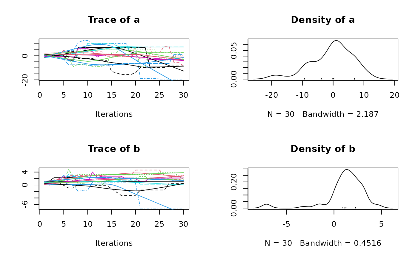
plot(res2$samples)


## use different evolution move, return samples as 'coda' object
res3 <- MCMCEnsemble(p.log, inits = unif_inits,
                     max.iter = 150, n.walkers = n_walkers,
                     method = "differential.evolution", coda = TRUE)
#> Using differential.evolution move with 10 walkers.

attr(res3, "ensemble.sampler")
#> [1] "differential.evolution"

summary(res3$samples)
#>
#> Iterations = 1:15
#> Thinning interval = 1
#> Number of chains = 10
#> Sample size per chain = 15
#>
#> 1. Empirical mean and standard deviation for each variable,
#>    plus standard error of the mean:
#>
#>    Mean    SD Naive SE Time-series SE
#> a 2.020 5.547   0.4529         0.8769
#> b 1.036 1.114   0.0910         0.1826
#>
#> 2. Quantiles for each variable:
#>
#>      2.5%     25%    50%   75%  97.5%
#> a -7.3644 -1.2012 0.9448 5.296 12.344
#> b -0.8414  0.3566 0.9145 1.709  2.909
#>
plot(res3$samples)
