Can estimations go beyond outside the range of the
inits?
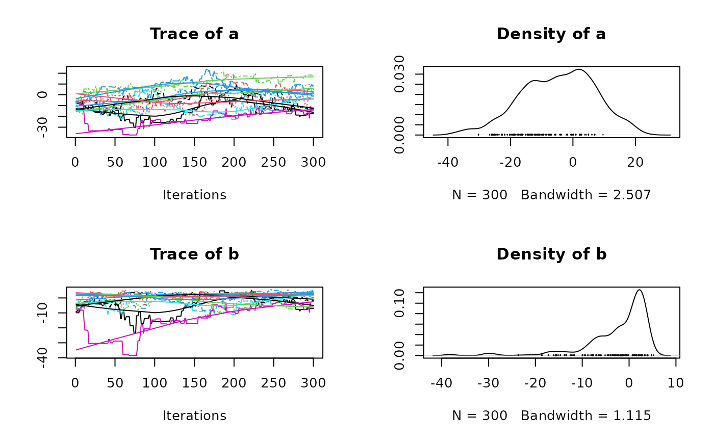
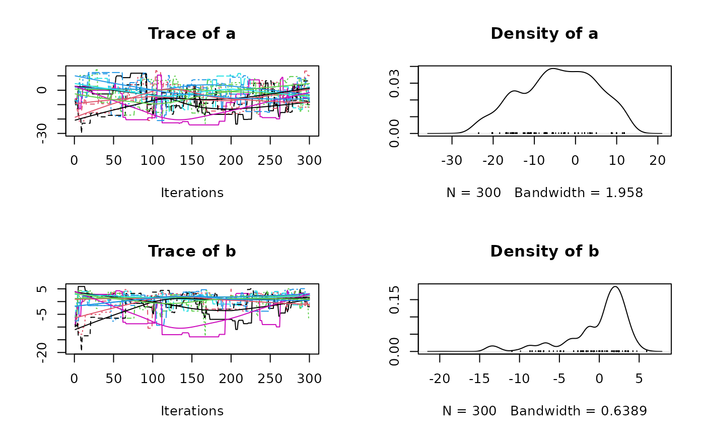
Yes, the inits and inits control the range
of the initial values, but the chain is still allowed to move
freely after this initial step, as shown in the following example.
Please report to the next question to learn how you can specify hard limits for the chains.
## a log-pdf to sample from
p.log <- function(x) {
  B <- 0.03 # controls 'bananacity'
  -x[1]^2 / 200 - 1 / 2 * (x[2] + B * x[1]^2 - 100 * B)^2
}

unif_inits <- data.frame(
  a = runif(10, min = -10, max = -5),
  b = runif(10, min = -10, max = -5)
)

set.seed(20201209)

res1 <- MCMCEnsemble(
  p.log,
  inits = unif_inits,
  max.iter = 3000, n.walkers = 10,
  method = "stretch",
  coda = TRUE
)
#> Using stretch move with 10 walkers.

summary(res1$samples)
#>
#> Iterations = 1:300
#> Thinning interval = 1
#> Number of chains = 10
#> Sample size per chain = 300
#>
#> 1. Empirical mean and standard deviation for each variable,
#>    plus standard error of the mean:
#>
#>     Mean     SD Naive SE Time-series SE
#> a -5.752 13.780   0.2516         1.3148
#> b -4.103  7.469   0.1364         0.6263
#>
#> 2. Quantiles for each variable:
#>
#>     2.5%    25%    50%   75%  97.5%
#> a -30.09 -17.02 -6.221 5.538 19.507
#> b -24.68  -7.90 -2.128 1.711  3.932
plot(res1$samples)
res2 <- MCMCEnsemble(
  p.log,
  inits = unif_inits,
  max.iter = 3000, n.walkers = 10,
  method = "differential.evolution",
  coda = TRUE
)
#> Using differential.evolution move with 10 walkers.

summary(res2$samples)
#>
#> Iterations = 1:300
#> Thinning interval = 1
#> Number of chains = 10
#> Sample size per chain = 300
#>
#> 1. Empirical mean and standard deviation for each variable,
#>    plus standard error of the mean:
#>
#>      Mean    SD Naive SE Time-series SE
#> a -0.8432 8.030  0.14661         0.6125
#> b  1.0343 2.286  0.04174         0.1609
#>
#> 2. Quantiles for each variable:
#>
#>      2.5%     25%     50%   75%  97.5%
#> a -14.461 -7.3898 -0.5432 5.457 13.256
#> b  -4.347 -0.2204  1.5516 2.673  4.224
plot(res2$samples)
How to restrict the possible parameter range?
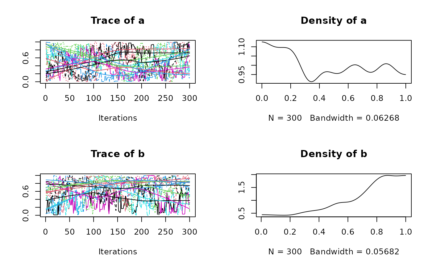
There is no built-in way to define hard limits for the parameter and make sure they never go outside of this range.
The recommended way to address this issue is to handle these cases in
the function f you provide.
For example, to keep parameters in the 0-1 range:
p.log.restricted <- function(x) {

  if (any(x < 0, x > 1)) {
    return(-Inf)
  }

  B <- 0.03 # controls 'bananacity'
  -x[1]^2 / 200 - 1 / 2 * (x[2] + B * x[1]^2 - 100 * B)^2
}

unif_inits <- data.frame(
  a = runif(10, min = 0, max = 1),
  b = runif(10, min = 0, max = 1)
)

res <- MCMCEnsemble(
  p.log.restricted,
  inits = unif_inits,
  max.iter = 3000, n.walkers = 10,
  method = "stretch",
  coda = TRUE
)
#> Using stretch move with 10 walkers.
summary(res$samples)
#>
#> Iterations = 1:300
#> Thinning interval = 1
#> Number of chains = 10
#> Sample size per chain = 300
#>
#> 1. Empirical mean and standard deviation for each variable,
#>    plus standard error of the mean:
#>
#>     Mean     SD Naive SE Time-series SE
#> a 0.4952 0.2811 0.005132        0.03139
#> b 0.6649 0.2446 0.004466        0.02832
#>
#> 2. Quantiles for each variable:
#>
#>      2.5%    25%    50%    75%  97.5%
#> a 0.02354 0.2621 0.4926 0.7373 0.9733
#> b 0.12695 0.4974 0.7093 0.8689 0.9894
plot(res$samples)
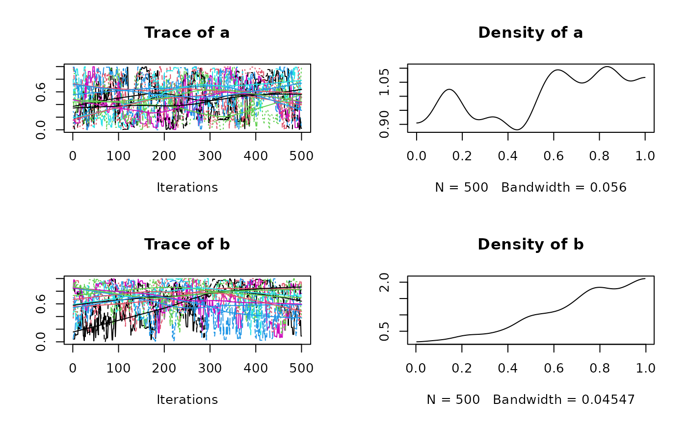
This might seem inconvenient but in most cases, users will define
their posterior probability as the product of a prior probability and
the likelihood. In this situation, values that are not contained in the
log-prior density automatically return -Inf in the
log-posterior and it is not necessary to define it explicitly:
prior.log <- function(x) {
 dunif(x, log = TRUE)
}

lkl.log <- function(x) {
  B <- 0.03 # controls 'bananacity'
  -x[1]^2 / 200 - 1 / 2 * (x[2] + B * x[1]^2 - 100 * B)^2
}

posterior.log <- function(x) {
  sum(prior.log(x)) + lkl.log(x)
}

res <- MCMCEnsemble(
  posterior.log,
  inits = unif_inits,
  max.iter = 5000, n.walkers = 10,
  method = "stretch",
  coda = TRUE
)
#> Using stretch move with 10 walkers.
summary(res$samples)
#>
#> Iterations = 1:500
#> Thinning interval = 1
#> Number of chains = 10
#> Sample size per chain = 500
#>
#> 1. Empirical mean and standard deviation for each variable,
#>    plus standard error of the mean:
#>
#>     Mean     SD Naive SE Time-series SE
#> a 0.4909 0.2908 0.004113        0.02486
#> b 0.7059 0.2435 0.003443        0.02487
#>
#> 2. Quantiles for each variable:
#>
#>      2.5%    25%    50%    75%  97.5%
#> a 0.03674 0.2337 0.4820 0.7462 0.9744
#> b 0.12457 0.5699 0.7736 0.9042 0.9922
plot(res$samples)